Some useful spreadsheet functions: FORMULATEXT, MATCH, CONCATENATE and INDIRECT

Tagged with spreadsheets
Posted 6 December 2019

I’ve been doing some work in spreadsheets recently, and I stumbled upon a couple of functions that let me do some neat things. I don’t do that much number crunching in Excel, so I’m leaving some notes here for my future self.

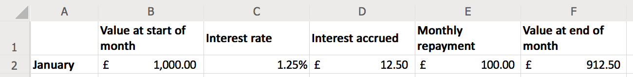
I was making a spreadsheet to track my student loan repayments, but this template could work for any sort of long-term loan. Here’s what my spreadsheet looks like:

A row of a spreadsheet with headings 'Value at start of month', 'Interest rate', 'Interest accrued', 'Monthly repayment', 'Value at end of month'.

The columns are as follows:

The value at the start of the month tells me how much I have to pay off at the start of the month.
The loan accrues interest every month, say at an interest rate of 1.25%. Multiply that by the current value of the loan, 1.25% of £1000 is £12.50, so that’s the interest accrued.
If I pay off £100 (the monthly repayment), then at the end of the month I have £1000 + £12.50 − £100 = £912.50 left to repay.

This is a fairly typical loan pattern. It doesn’t always exactly match the figures from the lender (for example, if they round in a slightly different way to me), but it’s close enough to be useful. I use these spreadsheets to get a rough idea of my finances, not exact predictions.

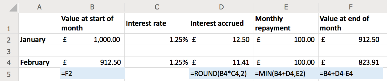
I can use Excel formulas to calculate the values in each row automatically, rather than calculating them by hand. Below each cell is the formula that created the result:

A row of a spreadsheet, with the formulae for each cell annotated in blue.

These are standard arithmetic:

=F2: The value at the start of one month is the same as the value at the end of the previous month.
=ROUND(B4*C4,2): The interest accrued is the current value of the loan multiplied by the interest rate. I round to 2 decimal places (the nearest penny) to keep the maths simple -- this avoids weird fractional pennies paying off in the background.
=MIN(B4+D4,E2): I pay off the same amount as the previous month, unless the total money left in the loan is less than my regular repayment. If I only have £50 left to repay, I shouldn't hand over £100.
=B4+D4-E4: At the end of the month, the total left on the loan is what I had at the start of the month, plus any interest I've accrued, less what I've repaid that month.

The blue cells contain the result of the first new function: FORMULATEXT. This returns the text of a formula as a string, rather than the result. For example, in cell B5 I have a formula =FORMULATEXT(B4). This looks in cell B4, then prints the formula it contains, which in this case is =F2.

I can imagine using this as a debugging tool, or if I wanted to show how a spreadsheet worked in a teaching example. It’s better than manually copying the formula text around, because it’s guaranteed to stay up-to-date.

Now suppose we let the loan run for a while. Hopefully the total amount goes down over time, and eventually it might get to zero:

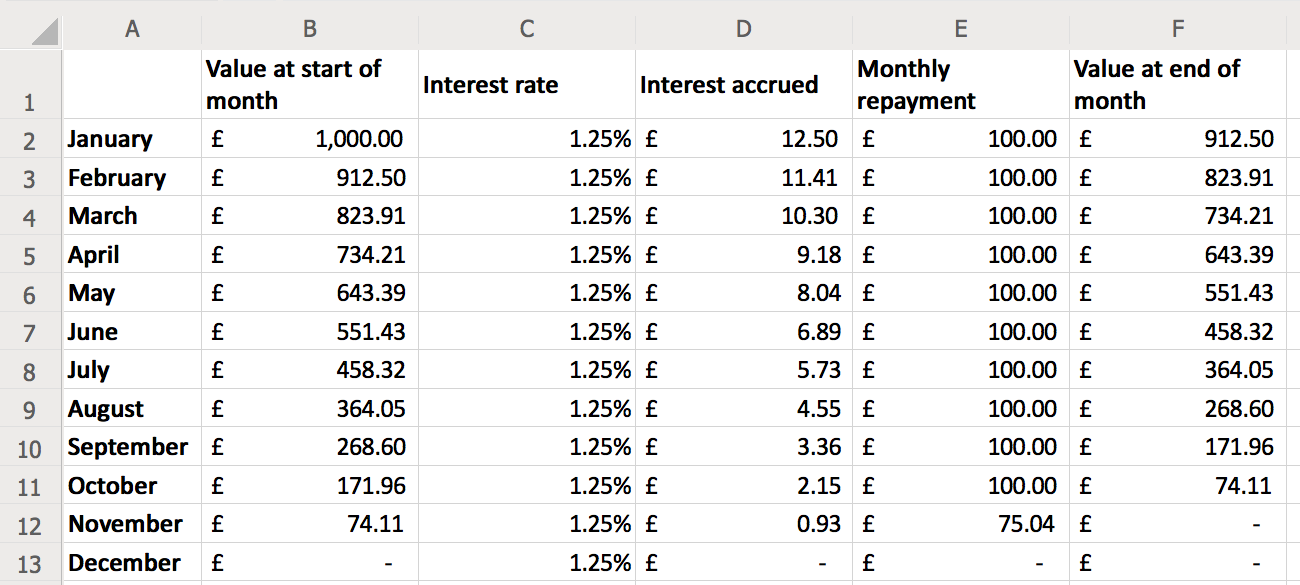
The spreadsheets above, but with rows from January to December.

Here the loan was fully paid off at the end of November. But if the loan hung around for longer, we might not fit all the rows on the screen – can we still find out when the loan finishes? Could the spreadsheet say “The loan will be fully paid off in November”, without us having to scroll down and find that ourselves?

It turns out there are a couple of formulas that can help us:

Some intermediate values, with their formulas shown in blue.

Here’s how they work:

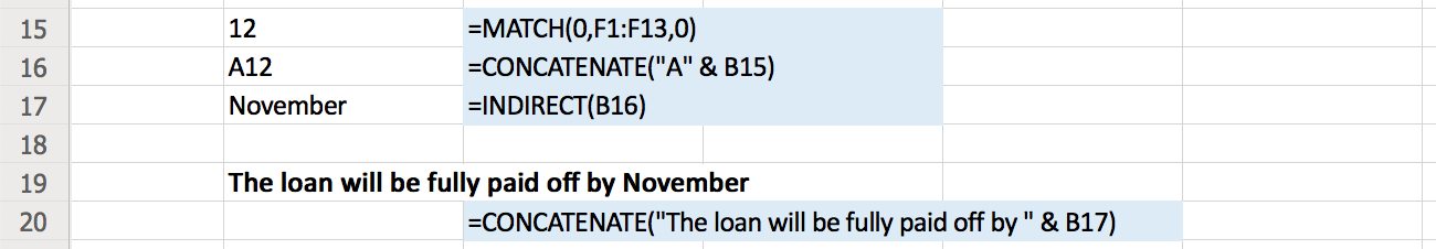
=MATCH(0,F1:F13,0): The MATCH function finds the first time a value appears in a collection — in this case, I’m telling it to find the first time a cell in the range F1:F13 has the value 0. (The value I'm looking for is the first argument; the third argument tells MATCH how to compare values in the cell range it’s checking.) In this case, it tells us that the 12th element in the range of cells – that is, the 12th row – is the first time the value at the end of the month is 0. So we know the 12th row is when the loan was paid off.
=CONCATENATE("A" & B15): Now we want to get the name of the month in row 12. The cell reference is A12, and we can build this reference with the CONCATENATE function. This function combines multiple strings – in this case, the literal string "A", and the result of the MATCH function in cell B15.
=INDIRECT(B16): If you have a cell reference as text, you can use the INDIRECT function to look up the contents of the cell. In this example, it first looks up the contents of cell B16 -- the literal string "A12", so it means =INDIRECT("A12"). Then the contents of cell A12 is the string "November", so that's what this function returns.

Calling the CONCATENATE function again gets me what I want: a sentence telling me when the loan will be finished. I can put this somewhere prominent, and the text will update as I tweak the parameters.

This has been useful for experimenting with some different repayment options – if I pay off more each month, does it change how much I pay, or how quickly I finish the loan? I can tweak some values, and instantly get those answers – not go hunting to find them.

It goes beyond just loan repayments – FORMULATEXT seems great for teaching, and CONCATENATE and INDIRECT allow a level of dynamic programming that I haven’t known how to do in Excel before. I don’t know when I’ll need spreadsheets again, but I’m excited to have these functions available when I do.

If you’d like to play with the spreadsheet I used for this post, you can download your own copy.