Getting a tint colour from an image with Python and k‑means
As part of my app for storing my electronic documents, there’s a grid view that displays big thumbnails of all my files. If I’m looking for something with a distinctive thumbnail (say, an ebook cover), I can easily skim a grid of thumbnails to find it. (I talked about how I create the PDF thumbnails in a separate post.)
When you hover over a card, it shows a little panel with some details about the file: when I saved it, how I’ve tagged it, and where I downloaded it from. Here’s a screenshot:
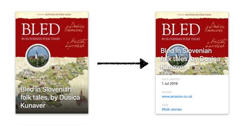
The source URL and tags are both clickable links. I can go back to the original page, or see other files with the same tags.
It’s a bit visually jarring to see the Bootstrap blue next to the large thumbnail. I wanted to see if I could pick a colour from the thumbnail, and use that for the link colour – for example, taking the bright red sash from the book cover above:
I’ve come up with an approach that seems to work fairly well, which uses k‑means clustering to get the dominant images, and then compares the contrast with white to pick the best colour to use as the tint. I’ve tried my code with a few thousand images, and it picks reasonable colours each time – not always optimal, but scanning the list I didn’t see anything wildly inappropriate or unusable.
Find the most common colour in an image?
My first thought was to try a very simple approach: tally all the colours used in the image, and pick the colour that appears most often.
The Pillow library has a getdata() method that lets you get a list of all the colours in an image, along with their frequency. So we can find the most common colour like so:
import collections

from PIL import Image


def get_colors_by_frequency(im):
    return collections.Counter(im.getdata())


if __name__ == "__main__":
    im = Image.open("cats.jpg")
    colors = get_colors_by_frequency(im)
    print(colors.most_common(1))
But if you actually try this, you quickly discover that it usually returns something close to black or close to white – it’s not very representative! (For scanned documents it’s almost always white.) Here’s an example:
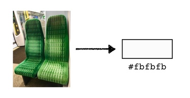
A human looking at that photo would probably pick green as the main colour – but there are lots of different shades of green. Although there are more green-ish pixels than any other colour, there are only a few of each exact shade, so they’re low down on the colour tally.
If we want to extract the main colours, we need to be able to group similar-looking colours together. We want to count all the different shades of green together.
I played with a couple of simple ideas, but I didn’t get anywhere useful, so I searched for other people tackling this problem. I found a post by Charles Leifer addressing a similar problem that suggested using k‑means clustering, so I decided to try that.
I’ve never used k‑means before, so I wanted to take time to understand it. There’s an implementation of k‑means in scikit-learn, but I wanted to write my own to be sure I really knew what was going on. If you already know how k‑means works, you can skip the next two sections – if not, read on, and I’ll do my best to explain.
What is k‑means clustering?
Suppose we have a collection of data points. Clustering means dividing the data points into different groups, so all of the points in each group are similar in some way. (And conversely, points in different groups should be different.)
For example, let’s suppose our data points are positions on a 2D plane. If we group them into three clusters by saying “points that are close together are similar”, we might end up with this clustering:
There are lots of ways to find clusters; k‑means is just one of them. It lets you group your data into k clusters, where k is a number you can choose.
Visual examples often help me understand something like this, and the Wikipedia article has some good illustrations. Let’s walk through them. Suppose we have some points in 2D space, and we want to divide them into 3 clusters:
Step 1: we start by picking 3 points at random. These are the initial “means”:
Step 2: go through all the points, and measure the distance from the point to each of the means. Put each point in a cluster with the closest mean, which divides the points into 3 clusters:
Step 3: within each cluster, calculate the centre, and use that as the new mean.
Because the means have moved, some of the points are now in the wrong cluster. They’re closer to the mean of a different cluster than the cluster they’re currently in. Re-run step 2 and step 3 until the clusters stop changing. This gives you the final 3 clusters:
To recap:
- Pick k points at random as the initial “means”.
- Put each point in a cluster with its closest mean.
- Calculate the centre of each cluster, and use that as the new mean.
- Repeat steps 2 and 3 until the clusters stop changing.
So how can we use this to find dominant colours in an image?
One way to represent colours is to treat them as a combination of red, green and blue components (RGB). We can treat these as positions in 3D space, and then use this algorithm – although the example above is in 2D, it extends readily to multiple dimensions. By grouping colours with this algorithm, we’ll end up with clusters of visually similar colours.
Implementing k‑means clustering for colours
As I said above, you can get a prebuilt implementation of k‑means from scikit-learn. I’m going to write one here as a learning exercise, and to make sure I really understand the algorithm, but you shouldn’t use this code for anything serious.
Let’s start by creating a class to represent a colour in RGB space (I’m using the attrs library here):
import attr


@attr.s(cmp=True, frozen=True)
class RGBColor:
    red = attr.ib()
    green = attr.ib()
    blue = attr.ib()
Step 1: pick k points at random as the initial means:
import random


def kmeans(colors, *, k):
    means = random.sample(colors, k)
    ...
Step 2: For each point, find the closest mean, and put that point in a cluster with that mean. We can use the Euclidean metric to measure the distance between two points. If you remember Pythagoras’ theorem from school, it’s the same idea in a more general form. (There are other ways to measure colour distance, but the distinction isn’t important for this exercise.)
import math


def euclidean_distance(color1, color2):
    return math.sqrt(
        (color1.red - color2.red) ** 2 +
        (color1.green - color2.green) ** 2 +
        (color1.blue - color2.blue) ** 2
    )


def kmeans(colors, *, k):
    ...
    clusters = {m: set() for m in means}

    for col in colors:
        closest_mean = min(
            means,
            key=lambda m: euclidean_distance(m, col)
        )

        clusters[closest_mean].add(col)

    ...
Step 3: Calculate the centre of each cluster, and use that as the new mean.
We use the arithmetic mean of all the points in the cluster as the centre. I’m also tracking how much the means change – by looking at this, we can tell when the clusters stop changing and when we can stop the process. This does a single pass:
def calculate_new_centre(colors):
    return RGBColor(
        red=int(sum(c.red for c in colors) / len(colors)),
        green=int(sum(c.green for c in colors) / len(colors)),
        blue=int(sum(c.blue for c in colors) / len(colors)),
    )


def kmeans(colors, *, k):
    ...

    new_means_distance = 0

    means = []

    for mean, colours_in_cluster in clusters.items():
        new_mean = calculate_new_centre(colours_in_cluster)
        means.append(new_mean)

        new_means_distance += euclidean_distance(mean, new_mean)
Now we repeat the process multiple times, until the means stop moving:
def kmeans(colors, *, k):
    means = random.sample(colors, k)

    while True:
        clusters = {m: set() for m in means}

        for col in colors:
            closest_mean = min(
                means,
                key=lambda m: euclidean_distance(m, col)
            )

            clusters[closest_mean].add(col)

        new_means_distance = 0

        means = []

        for mean, colours_in_cluster in clusters.items():
            new_mean = calculate_new_centre(colours_in_cluster)
            means.append(new_mean)

            new_means_distance += euclidean_distance(mean, new_mean)

        if new_means_distance == 0:
            return means
It hands back the means – the centres of each cluster – as a representative of all the colours in that cluster. This is what I’ll be using for a tint colour later.
This code assumes that the clusters eventually stop moving – if not, it’ll spin forever in an infinite loop. When I tried this on some of my images, the colour clusters converged pretty quickly with k = 3 and k = 5, but that may not be true in the general case.
Putting all that code together, here’s the final version:
import math
import random

import attr


@attr.s(cmp=True, frozen=True)
class RGBColor:
    red = attr.ib()
    green = attr.ib()
    blue = attr.ib()


def euclidean_distance(color1, color2):
    return math.sqrt(
        (color1.red - color2.red) ** 2 +
        (color1.green - color2.green) ** 2 +
        (color1.blue - color2.blue) ** 2
    )


def calculate_new_centre(colors):
    return RGBColor(
        red=int(sum(c.red for c in colors) / len(colors)),
        green=int(sum(c.green for c in colors) / len(colors)),
        blue=int(sum(c.blue for c in colors) / len(colors)),
    )


def kmeans(colors, *, k):
    """
    Find the result of a k-means clustering over ``colors``.

    :param k: The number of clusters to create.

    """
    # Choose k points at random as the initial means.
    means = random.sample(colors, k)

    while True:
        # For each point, find the closest mean, and put that point in
        # a cluster with that mean.
        clusters = {m: set() for m in means}

        for col in colors:
            closest_mean = min(
                means,
                key=lambda m: euclidean_distance(m, col)
            )

            clusters[closest_mean].add(col)

        # Calculate the centre of each cluster, and use that as the
        # new mean.
        new_means_distance = 0
        means = []

        for mean, colours_in_cluster in clusters.items():
            new_mean = calculate_new_centre(colours_in_cluster)
            means.append(new_mean)

            new_means_distance += euclidean_distance(mean, new_mean)

        # If the means have stopped changing, then the clusters have
        # converged, and we can terminate.
        if new_means_distance == 0:
            return means
If you want to do something similar with scikit-learn, you can do:
from sklearn.cluster import KMeans


def kmeans(colors, *, k):
    return KMeans(n_clusters=k).fit(colors).cluster_centers_
Now we have a way to extract dominant colours from an image, let’s return to the problem of finding tint colours.
Picking a tint colour from the dominant colours
We can use our k‑means clustering algorithm to extract dominant colours from an image. Combining it with the code to extract all the pixels with Pillow:
from PIL import Image
from sklearn.cluster import KMeans


def get_dominant_colours(path, *, count):
    im = Image.open(path)
    colors = im.getdata()

    return KMeans(n_clusters=count).fit(colors).cluster_centers_
The k‑means clustering gives us a way to extract some dominant colours from an image; here’s the example of the green chair above with 3 means and 5 means:
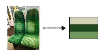
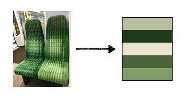
Those colours are much more representative than a bright white or dark black.
Now we need to pick which of those to use as a tint colour for the text to accompany this image. A good choice will vary based on the context – a dark tint colour works well on a white background, but you’d want the opposite for a black background.
Computing the dominant colours is (relatively) slow – it took several minutes to run the k‑means clustering for 1000 images on my six-year-old iMac. I picked k = 5 mostly arbitrarily, and cached the results in a JSON file. Then I experimented with different tint colour pickers on the cached data, and created a script that would show me what colours it had picked:
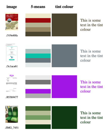
I played with various approaches: picking the colour with the biggest cluster size, trying to maximise or minimise distance from white in the RGB space, filtering by lightness in the HSL colour space. Nothing quite looked right – some approaches would always pick the really dark colours (which is less visually interesting), or sometimes pick an inappropriately light colour (which is hard to read).
Eventually I struck upon the idea of using WCAG contrast ratios. The WCAG recommends a minimum contrast ratio of 4.5:1 for displaying text on a web page, so the first step is to throw away all colours that don’t have sufficient contrast with the background. There’s a Python library that computes these ratios for you, so let’s use that:
import wcag_contrast_ratio as contrast


def choose_tint_color(dominant_colors, background_color):
    sufficient_contrast_colors = [
        col
        for col in dominant_colors
        if contrast.rgb(col, background_color) >= 4.5
    ]
Two of the images in my test set don’t have any dominant colours that pass WCAG with a white background – as a quick workaround, add black and white to the mix and try again (every colour has a contrast ratio of 4.5:1 with at least one of black or white; see proof):
def choose_tint_color(dominant_colors, background_color):
    ...

    if not sufficient_contrast_colors:
        return choose_tint_color(
            dominant_colors=dominant_colors + [(0, 0, 0), (1, 1, 1)],
            background_color=background_color
        )
You could do something more interesting here, but it didn’t seem worth the effort. I considered fuzzing the dominant colours until the contrast was sufficient for one of them, but that adds a lot of complexity for something that affects a tiny fraction of my images.
So now we have some colours we could use and meet contrast requirements, but which would be the best to use? This is mostly down to aesthetic preference – what looks good to you?
If you max out the contrast ratio, the tints tend towards the very dark or very light colours. I’d prefer something a bit brighter, more colourful, so I tried converting the colours to the HSL (hue, saturation, lightness) space, and picking the colour with the closest lightness to the background. That means I get something with sufficient contrast but that isn’t too dark or too light.
Handily, Python includes the colorsys module, which lets you convert between the RGB and HSL colour spaces (although the module calls it HSV). Like so:
import colorsys


def choose_tint_color(dominant_colors, background_color):
    ...

    hsv_background = colorsys.rgb_to_hsv(*background_color)
    hsv_candidates = {
        rgb_col: colorsys.rgb_to_hsv(*rgb_col)
        for rgb_col in sufficient_contrast_colors
    }

    candidates_by_brightness_diff = {
        rgb_col: abs(hsv_col[2] - hsv_background[2])
        for rgb_col, hsv_col in hsv_candidates.items()
    }

    rgb_choice, _ = min(
        candidates_by_brightness_diff.items(),
        key=lambda t: t[1]
    )

    assert rgb_choice in dominant_colors
    return rgb_choice
I’ve run this over about 1000 images from my photo library, and checked the tints with my viewer script:
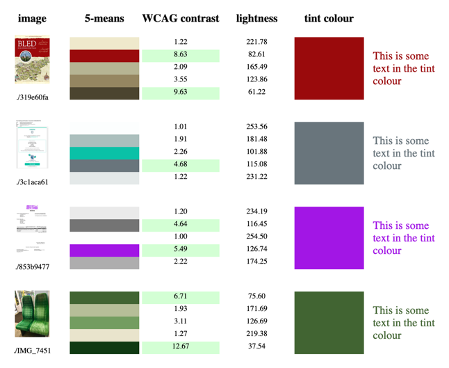
It usually picks a sensible tint – enough contrast, a colour that comes from the original image, and somewhat visually interesting. It doesn’t always pick the “best” colour (or at least, what I’d have picked), but the combination of WCAG contrast ratio and minimising the lightness difference means it never picks something bad. The colours it selects are never visually jarring.
Putting it all together
This is the complete code, wrapped in a script that lets you run it standalone against an image:
#!/usr/bin/env python
# -*- encoding: utf-8

import colorsys

from PIL import Image
from sklearn.cluster import KMeans
import wcag_contrast_ratio as contrast


def get_dominant_colours(path, *, count):
    """
    Return a list of the dominant RGB colours in the image at ``path``.

    :param path: Path to the image file.
    :param count: Number of dominant colours to find.

    """
    im = Image.open(path)

    # Resizing means less pixels to handle, so the *k*-means clustering converges
    # faster.  Small details are lost, but the main details will be preserved.
    im = im.resize((100, 100))

    # Ensure the image is RGB, and use RGB values in [0, 1] for consistency
    # with operations elsewhere.
    im = im.convert("RGB")
    colors = [(r / 255, g / 255, b / 255) for (r, g, b) in im.getdata()]

    return KMeans(n_clusters=count).fit(colors).cluster_centers_


def choose_tint_color(dominant_colors, background_color):
    # The minimum contrast ratio for text and background to meet WCAG AA
    # is 4.5:1, so discard any dominant colours with a lower contrast.
    sufficient_contrast_colors = [
        col
        for col in dominant_colors
        if contrast.rgb(col, background_color) >= 4.5
    ]

    # If none of the dominant colours meet WCAG AA with the background,
    # try again with black and white -- every colour in the RGB space
    # has a contrast ratio of 4.5:1 with at least one of these, so we'll
    # get a tint colour, even if it's not a good one.
    #
    # Note: you could modify the dominant colours until one of them
    # has sufficient contrast, but that's omitted here because it adds
    # a lot of complexity for a relatively unusual case.
    if not sufficient_contrast_colors:
        return choose_tint_color(
            dominant_colors=dominant_colors + [(0, 0, 0), (1, 1, 1)],
            background_color=background_color
        )

    # Of the colours with sufficient contrast, pick the one with the
    # closest brightness (in the HSV colour space) to the background
    # colour.  This means we don't get very dark or very light colours,
    # but more bright, vibrant colours.
    hsv_background = colorsys.rgb_to_hsv(*background_color)
    hsv_candidates = {
        tuple(rgb_col): colorsys.rgb_to_hsv(*rgb_col)
        for rgb_col in sufficient_contrast_colors
    }

    candidates_by_brightness_diff = {
        rgb_col: abs(hsv_col[2] - hsv_background[2])
        for rgb_col, hsv_col in hsv_candidates.items()
    }

    rgb_choice, _ = min(
        candidates_by_brightness_diff.items(),
        key=lambda t: t[1]
    )

    assert rgb_choice in dominant_colors
    return rgb_choice


if __name__ == "__main__":
    import sys

    try:
        path = sys.argv[1]
    except ImportError:
        sys.exit(f"Usage: {__file__} <PATH>")

    dominant_colors = get_dominant_colours(path, count=5)
    tint_color = choose_tint_color(dominant_colors, background_color=(0, 0, 0))

    print(tint_color)
    print("#%02x%02x%02x" % tuple(int(v * 255) for v in tint_color))
I haven’t integrated it into docstore yet, but that should be the easy bit – finding a good way to pick tint colours was where I struggled before.
When I do use this code, I’ll cache the k‑means results and compute the tint colours on the fly. The k‑means results take a while to create and they shouldn’t change. Caching those results will make it easier for me to keep tweaking the function that picks the tint colour, if/when I get more ideas.
When I wrote the original version of this code on Thursday night, it was right at the limit of my understanding. It worked, but it was spaghetti code with a lot of unnecessary pieces that I could barely follow. Writing it out in detail has helped me understand why it works, the key ideas, and why it works better than my other attempts. The new code is also a lot clearer to read.
I hope you found this post interesting, and maybe it gave you some ideas for your own code. But the main value for me is better understanding of this tricky code, which will make it easier for me to maintain and update it in the future. If you’re ever struggling with a bit of code, I really can recommend writing it out in detail as a way to understand it better.